Training a YOLOv8 Object Detector

If you want to teach a model to spot things in pictures, then object detection is probably what you’re looking for. Computer vision isn’t exactly anything new, but YOLOv8 is leaps and bounds better than earlier versions I used in the past, which makes this interesting.

To help explain the process, let’s walk through the process of training a custom YOLOv8 object detector for Heavy Goods Vehicles (HGVs). You can train it for any type of object, I’m just choosing HGVs because of their relevance to my day-to-day job.

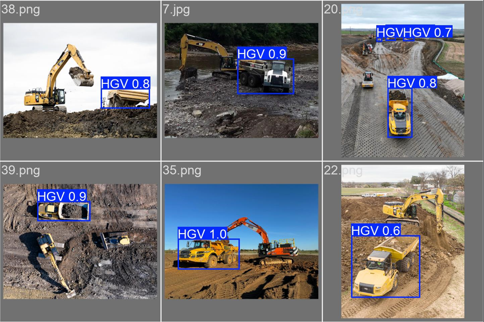
The end output should be a model that’s capable of identifying your trained object in a range of different images. Check out the below screenshot which shows how the trained model performs. In case you’re not sure of the significance of what you’re looking at – it’s the blue bounding boxes that have been automatically placed around each identified HGV by the model.

This looks impressive, but what can we actually do with this output? Is it even useful?

Yes! The ability to do this enables several relevant applications to be built:

1. Traffic monitoring and management: The model can count and track HGVs on highways, helping authorities manage traffic flow and plan infrastructure improvements.
2. Safety and compliance: If you identify HGVs in real-time, you can monitor their adherence to designated routes, speed limits, and restricted areas etc.
3. Parking management: Use it to identify available parking spaces for HGVs in rest areas or construction compounds, providing useful real-time data that can make resource allocation decisions.
4. Accident prevention and investigation: If you also train the model to identify workers, you can use the model to flag up instances when a HGV is near a worker. Couple this with other data, like vehicle speed, and it can be a powerful alerting system that can be used to improve on-safety arrangements.

Understanding Object Detection

Before we get into the details, it would be worth clarifying what object detection actually is first. Unlike image classification, which simply identifies what’s in an image, object detection locates and classifies multiple objects within an image. It answers two questions: “What objects are in this image?” and “Where are they located?”

YOLO (You Only Look Once) is a family of real-time object detection models, with YOLOv8 being one of its best iterations in terms of accuracy. YOLO is arguably one of the most well-known object detection models, and its strength lies in its ability to process images quickly while maintaining high accuracy, making it ideal for real-time applications.

1. First up: Collecting your Data

The first step in any machine learning project is data collection. As the saying goes, “garbage in, garbage out” – the quality of your data directly impacts your model’s performance.

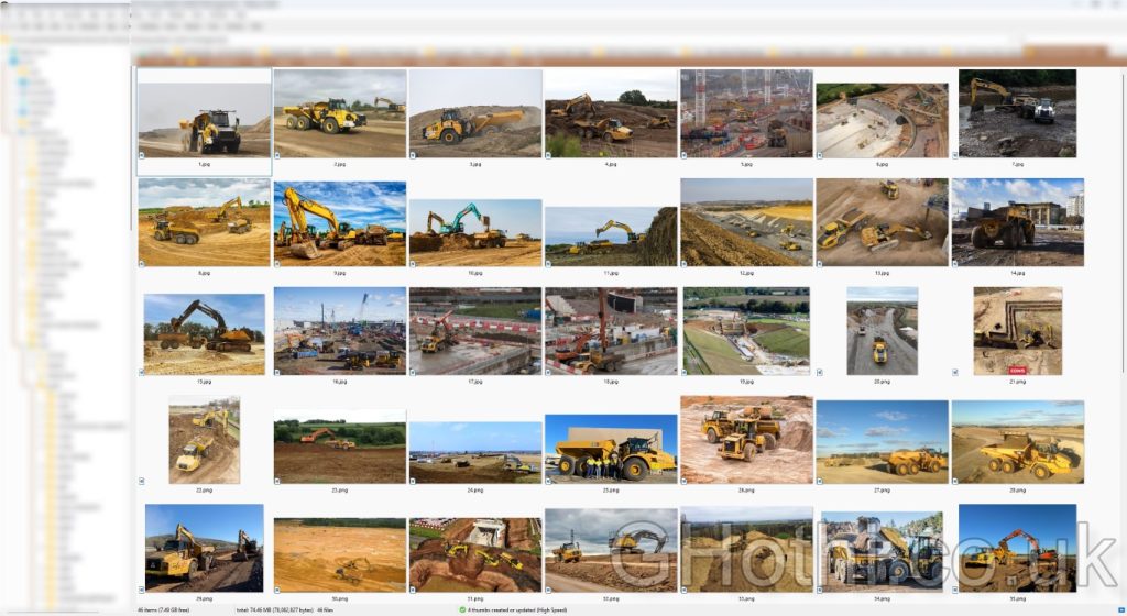
For our YOLOv8 custom detector, I’ve collected a small dataset of 50 HGV images from Google images, focusing on earthwork civil engineering projects.

In reality, you’d want much more than 50 images, and depending on what you plan to use the final model for, you’ll need to check what the specific copyright rules are for you. Seeing as I’m just training this as a quick non-commercial demo, there’s no real ‘practical’ harm from using Google to source these images.

Why Data Diversity Matters

Having a diverse dataset helps your model generalise better. For example, if all your HGV images are taken on sunny days, your model might struggle to detect HGVs in different weather conditions. Because of this, you should include images that cover a wide range of scenarios. In this case, think along the lines of varying:

• Lighting conditions (sunny, cloudy, nighttime)
• Backgrounds (construction sites, highways, quarries)
• Angles (front view, side view, aerial view)
• State (colours, tipper up, tipper down)
• Occlusions (partially hidden HGVs)

This diversity helps your model learn the actual features that define an HGV, rather than incidental features like “yellow color” or “dusty background”.

2. Data Annotation: Giving Context to Your Images

Once you’ve your images, the next step is annotating them. This step tells your model what to look for and where.

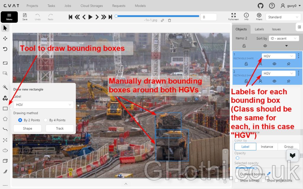
This process involves drawing bounding boxes around the HGVs in each image. There’s a ton of different tools for this, some free and some paid. You can even outsource this to a 3rd party and they’ll annotate your dataset for you!

I personally prefer using CVAT (Computer Vision Annotation Tool) for this because it’s free for what we’d need to use it for, has a clean GUI and is cloud-based, meaning there’s nothing to install on your PC.

Here’s a quick guide to using CVAT:

1. Create a new project and task

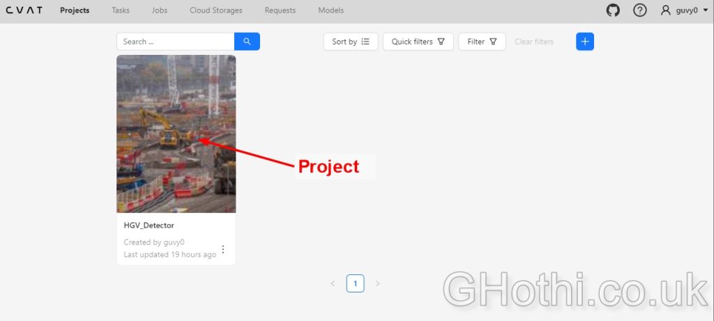
2. Upload your 50 HGV images to the task

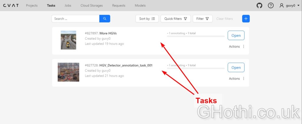
3. For each image, drawing bounding boxes around each HGV

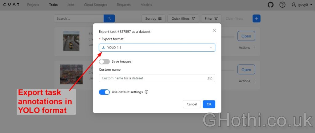
5. Save the task and export the annotations in YOLO format

The Importance of Accurate Annotations

Annotations are crucial because they teach the model what to look for and where. Think of them as the “ground truth” that your model will try to replicate. Poor annotations can confuse your model and lead to poor performance.

When drawing bounding boxes:

• Be consistent in how tightly you draw boxes around HGVs
• Include the entire vehicle, even if partially occluded
• Be careful with overlapping vehicles

Remember, your model will learn from these annotations, so accuracy here directly impacts your final model’s performance.

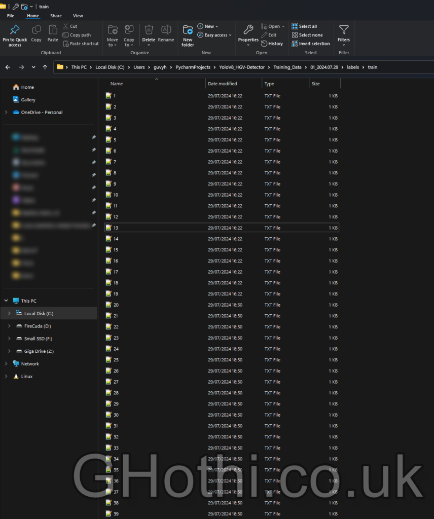
3. Data Formatting: Preparing for YOLOv8

YOLOv8 requires a specific data format. Here’s how to structure your data:

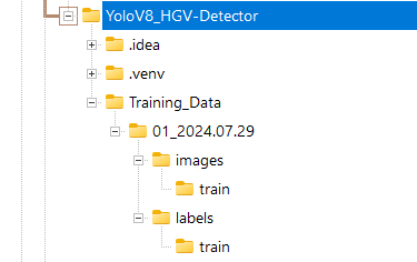
1. Create two main folders: ‘images’ and ‘labels’
2. Place all your 50 HGV images in the ‘images’ folder
3. Place the corresponding annotation files in the ‘labels’ folder that you downloaded from the previous step.

Each annotation file should be a .txt file with the same name as its corresponding image. For example:

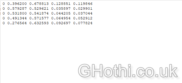
The content of each file should be in the format:

<class> <x_center> <y_center> <width> <height>

All values should be normalised to be between 0 and 1 (as they are relative to the image size).

For example, here’s a preview of the one the text files’ contents:

Understanding YOLO Format

The YOLO format might seem cryptic at first, but it’s quite efficient once you understand it. Here’s what each value means:

• <class>: An integer representing the object class (e.g., 0 for HGV)
• <x_center> <y_center>: The center coordinates of the bounding box, normalised by the image width and height
• <width> <height>: The width and height of the bounding box, also normalised

Normalisation (scaling values between 0 and 1) helps the model process images of different sizes consistently.

Next, create a new python project folder (I use PyCharm, but any python IDE is fine). Inside the project golder, create a configuration file named config.yaml with the following structure:

path: /path/to/your/dataset
train: images/train
val: images/val

names:
  0: HGV

Adjust the paths and class names according to your specific dataset.

What does the Configuration File do?

The config YAML file passes information to the training process. It tells YOLOv8:

• Where to find your dataset
• Which images to use for training and validation
• What classes you’re trying to detect

Separating training and validation sets is important because the validation set helps assess how well your model generalises to unseen data, preventing overfitting. Given I’m just running this as a quick test and my starting dataset is tiny, I decided not to provide an validation images as I’ll just test it myself manually afterwards. As a general rule, you want to reserve about 20% of your images as a validation set, but this really depends on the size of your dataset to start with. I like to use the following as a rule of thumb, with the latter numbers being more ideal:

• Datasets with 1000+ images: 10-20% for validation
• Datasets with 500-1000 images: 5-10% for validation
• Datasets with less than 500 images: Likely use cross-validation or a very small validation set (3-5%)

4. Model Training: Bringing Your Detector to Life

Now comes the exciting part – training your YOLOv8 model! First, ensure you have the ultralytics library installed:

pip install ultralytics

Then, create a Python script for training:

from ultralytics import YOLO

# Load a model
model = YOLO('yolov8n.yaml')  # build a new model from YAML

# Train the model
results = model.train(data='config.yaml', epochs=200, imgsz=640)

This script loads the YOLOv8 nano model and trains it on our custom HGV dataset for 100 epochs with an image size of 640x640. Feel free to adjust these parameters based on your specific needs and computational resources.

Understanding Key Training Parameters

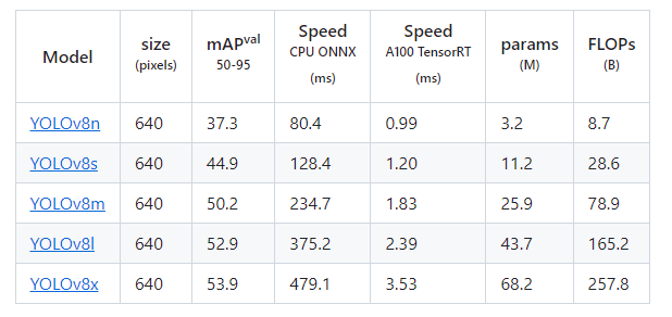
• Model Selection: ‘yolov8n.yaml’ refers to the “nano” version of YOLOv8. It’s the smallest and fastest model, but less accurate than larger versions like ‘yolov8l’ (large) or ‘yolov8x’ (extra large). Details of each model are shown above.
  I usually settle with yolov8m as it’s a nice middle ground between speed and quality. I personally find the ‘returns’ drop off beyond this medium model size. But for something being used in production stage, it’s definetly worth testing out the larger models as it could make the difference between your model being useful and useless when accuracy is a non-negotiable (i.e. if the model is being used to improve site-safety).
• Epochs: An epoch is one complete pass through your entire training dataset. More epochs allow for more learning but risk overfitting.
  Ultralytics, the creators of YOLOv8, recommend starting with 300 epochs for multi-class datasets.
  Don’t be afraid to experiment with different epoch sizes. You can start with the recommended 300 epochs and then adjust based on your specific results.
• Image Size: Larger sizes (e.g., 640×640) can improve accuracy for detecting small objects but require more computational resources. Smaller sizes are faster but may miss fine details.

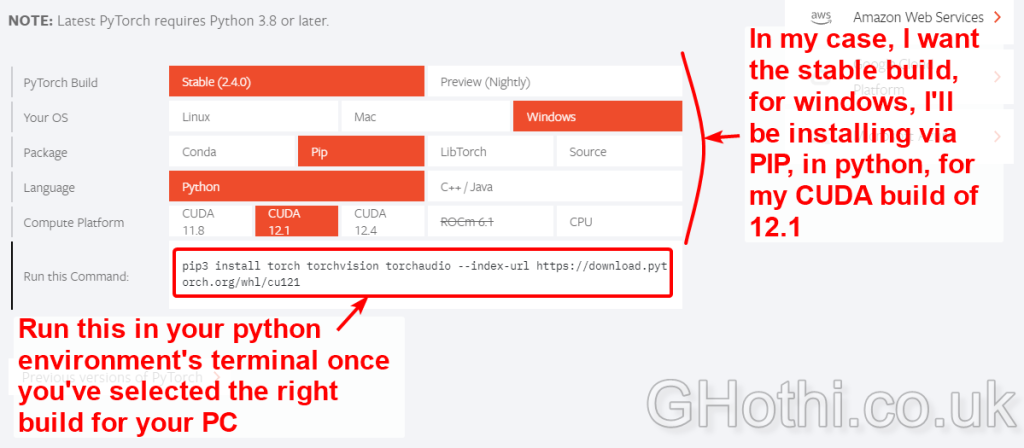
Note: Make sure you have PyTorch and CUDA installed on your PC to help speed up the training, otherwise you’ll be training the model using your CPU, which will be significantly slower! Setting up the right PyTouch and CUDA configuration can be a pain in the ass sometimes, so make sure you take a note of what configuration you used so you can use it for future projects.

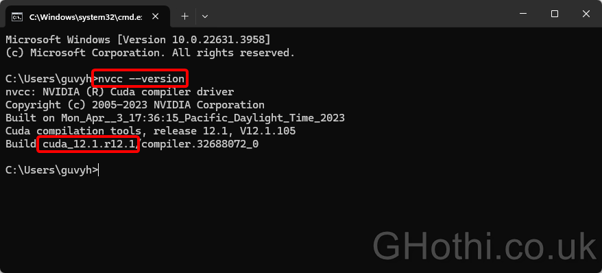
You’ll need to make sure you instal the right Torch build for your CUDA build. You can check your CUDA build using “nvcc –version” in the CMD window if you suspect you already have it installed.

With this info in mind, download the right PyTorch build from here: https://pytorch.org/

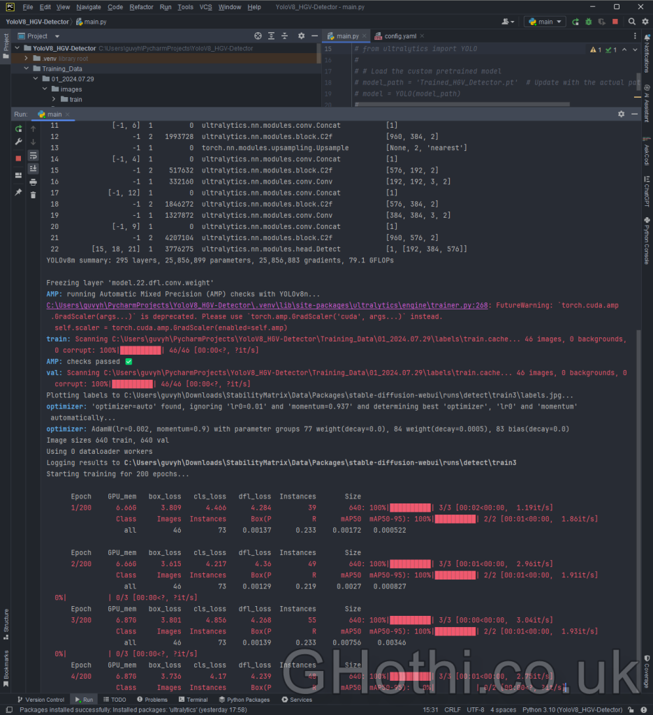
Now run this script, and YOLOv8 will start training. It should look something like the below, with real-time updates on each epoch’s progress during the training. The terminal shows a lot of detail at this stage, but we can review the most important ones after the training process, as it also spits them out in nice graphs which are easier to read.

5. Evaluating Model Performance: How Good Is Your Detector?

After training, you’ll be provided with a link to the output directory. The output folder will include the model and useful data that we can use to evaluate the model’s performance.

As a minimum, you’ll want to check:

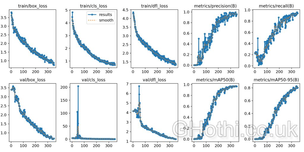
1. Loss Curves: Check if your training and validation losses are decreasing. This indicates that your model is learning.
2. Metrics: Look at mAP (mean Average Precision).
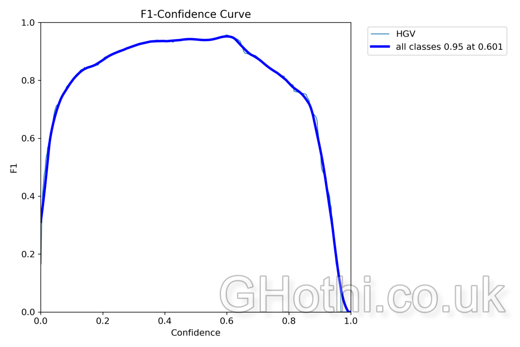
3. Visualization: YOLOv8 generates visualisations like confusion matrices and F1-confidence curves. Check these as well.

How Do You Read these Evaluation Metrics?

• Loss Curves: The loss is a parameter that reports how far the model’s predictions are from the actual data – it’s the loss function that actually guides it and tells it how it needs to improve during the ‘learning’ process.
  The aim of training is to minimise the loss of function.
  The curves shows you the loss at each training step. The important thing is to check that the loss is trending downwards.
  If it levels off for quite a few steps, you may start falling into over-training territory, and if it’s still falling quite rapidly (i.e. it still has a steep gradient), you may be in the under-training territory.
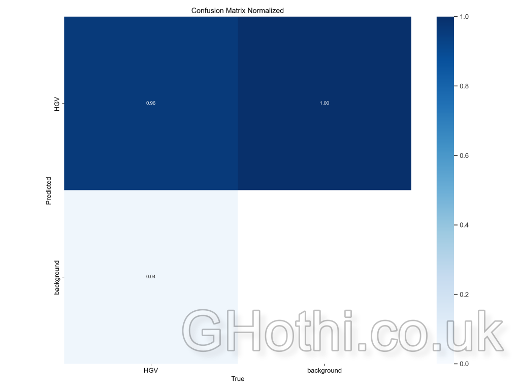
  Use this info to determine if you need to rerun the training with a reduced or increased number of epochs.
• Confusion Matrix: Shows how well the model’s predictions match the true labels for each class. It’s a 2×2 grid in this case, with the rows representing the predicted classes and the columns representing the actual classes.
  High values on the diagonal (top-left and bottom-right) indicate correct predictions. For example, a high value in the top-left cell means the model correctly predicted the presence of the HGV class.
  High values off the diagonal (top-right and bottom-left) indicate misclassifications. For example, a value in the bottom-left cell means the model incorrectly predicted the background when the actual class was HGV.
• F1 Score: The relationship between the model’s confidence in its predictions and the F1 score, which is a measure of a test’s accuracy. A higher and broader peak suggests that the model performs well over a range of confidence levels.
• mAP (mean Average Precision): This is a single number that summarises the model’s performance across all classes and detection thresholds. Higher is better.

Real-World Testing

The most important test is how your model performs on new unseen data. If it’s great at predicting the original dataset and not new images, then it means the training was unsuccessful, no matter how great the earlier evaluation metrics were.

To truly test your model, you need to run it on new images or videos to see how it performs in real-world scenarios.

To do this, locate your custom model, move it into your project folder along with some test images/videos, and run the model on each one of them and plot the results. You’ll have to write a basic script to run each image through the model, for example:

# Import the necessary module
from ultralytics import YOLO

# Load the custom pretrained model
model_path = 'Trained_HGV_Detector.pt'  # Update with the actual path to your model
model = YOLO(model_path)

# Load and run inference on an image
image_path = 'test_2.jpg'  # Update with the actual path to your image
results = model(image_path)

# Display the results
for result in results:
    result.plot()  # This will plot the results on the image
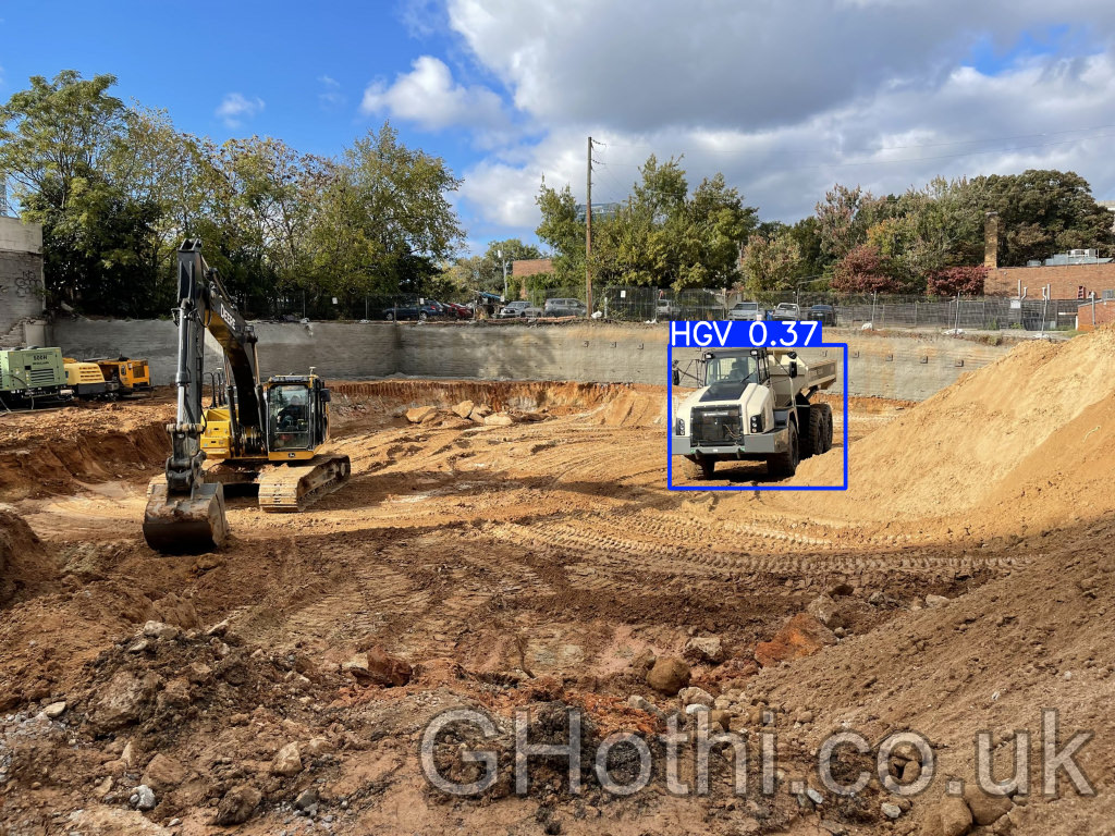
    result.show()  # This will display the plotted image

Here’s the first example of running an unseen image against the custom model:

And here’s the second example of running another unseen image against the custom model:

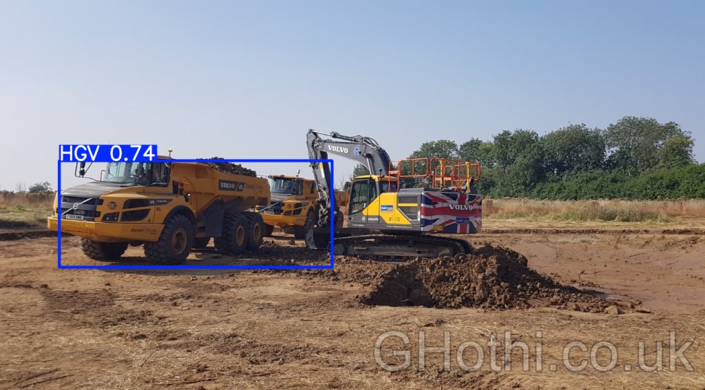
Surprisingly, the model works very well given the tiny dataset! However, the prediction in the 2nd example could definitely be better. Although it found and bounded both HGVs, it didn’t identify them as being two separate objects.

This means I need to expand the training dataset to include more examples of where one HGV partially occludes another. With a larger dataset and a few more of these specific occlusion images, it would likely do a much better job of predicting these. But just from a small dataset of 50 images and a bit of machine learning, we’ve been able to detect HGVs in different positions and environments with relatively good accuracy!

6. Iterative Improvement: Refining Your Model

Machine learning is an iterative process. If you’re not satisfied with your model’s performance, consider the following strategies:

1. Increase Training Time: Train for more epochs to allow your model to learn more complex features.
2. Adjust Hyperparameters: Experiment with different batch sizes, learning rates, or model architectures.
3. Augment Your Dataset: Add more diverse images or use data augmentation techniques to increase the variety in your training data. This is especially important given our small dataset of only 50 images.
4. Refine Your Annotations: Review and improve your annotations, ensuring they’re consistent and accurate.

Expanding your Dataset

What do you do if you can’t find enough images for your dataset? Thankfully, there’s a smart solution to this. It involves artificially expanding your dataset by creating modified versions of your existing images through operations like:

• Rotating
• Flipping
• Adjusting brightness and contrast
• Adding noise

This helps your model learn to be invariant to these changes, improving its performance in real-world scenarios.

Nothing beats having more unique images because of the amount of ‘new’ insight it offers, so you should only really rely on this step once you’ve exhausted other solutions.

Summary

Training a custom YOLOv8 object detector can open up a lot of possibilities in civil engineering and construction management. The applications really are only limited by your imagination (and dataset!)

Don’t be discouraged if your first attempt isn’t perfect – each iteration brings you closer to a high-performing model. It took me about 3 iterations of cranking my number of training epochs until I finally started getting some meaningful output.

Happy training!